Kernelized Support Vector Machine
Introduction
As introduced, Linear Support Vector Machine (Linear SVM) is a technique that can find an optimal hyperplane that can categorize data points into separate classes. Since reality is a complex endeavour, there would often be dataset that is not linearly separable. Kernel SVM is an extension of linear SVM technique in which it maps the input dataset into a higher dimensional plane (could be infinite). In this new high dimensional plane, the data is linearly separable. This transformation allows Kernel SVM to handle complex, nonlinear classification tasks efficiently. Depending on the kernel function used, it captures complex patterns and relationships in the data that a linear SVM might be unable to. Some popular kernel functions are Linear, Polynomial, Radial Basis Function, and Sigmoid. The selection of an appropriate kernel function and its parameters plays a crucial role in the perfomance of a Kernel SVM.
The kernel trick
In brief, Kernel SVM uses a transforming function \(\phi(x)\) that can transform the input data x from the original feature space into a new space. This function needs to sastify the purpose: in the new space, the dataset of the two classes are linearly separable or almost so. Then we can use the usual binary classifiers such as perceptron, logistic regression or hard/soft linear SVM.
Here is an example of a non linearly separable 1D dataset:
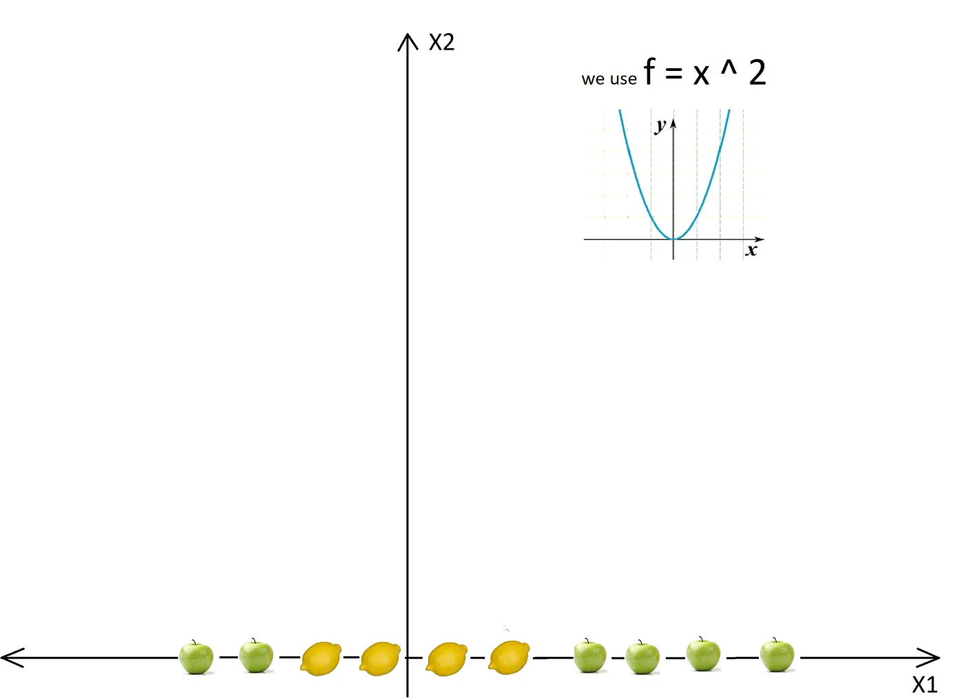
The dataset becomes separable with a line after converting to 2D:
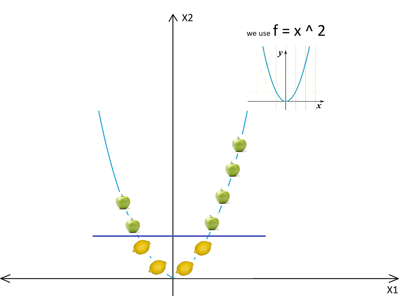
Importing the whole dataset into the higher dimensional space would be comptutational expensive. The reasonable thing to do is to define a kernel function that can return a measure of similarity (the inner product) of the images in the new space of any two input datapoints. After the transformation, SVM proceeds to find the hyperplan that can separate the data into distinct classes. The only difference is that the separation now happens in the higher dimensional space.
The kernel functions need to have some properties to be used. First, it needs to be symmetric \(k(x,y) = k(y,x)\) since the inner product of two vectors is symmetric. Second, it needs to fulfill the Mercer condition:
\[\sum_{n=1}^N \sum_{m=1}^N k(x_m, x_n) c_n c_m \geq 0, \forall c_i \in R, i = 1,2..N\]This condition is to make sure that the duality function of SVM to be convex. In reality, some kernel functions k doesn’t satisfy this condition but it is still acceptable. Third, the function k needs to be positive semi-definite:
\[\sum_{i=1}^n \sum_{j=1}^n c_i c_j k(x_i,x_j) \geq 0\]with \(x_i\) to be any point in the input space and \(c_i \in R\). This is to make sure that the Gram matrix (the matrix produced by taking the kernel of every pair of points in a set) has all non negative eigenvalues.
These properties is to ensure that the kernel function k can be expressed as a dot product in a higher dimensional feature space. Only then we can use linear methods for the high dimensional space.
Linear kernel
\[k(x,y) = x^T y\]The linear kernel is the simplest form of kernel function. It computes a linear combination of the input features, creating a linear decision boundary. x and y are vectors in the input space and x would be transposed before multiplying with y. The advantage of a linear kernel is its simplicity and speed. This is so because it doesn’t involve any additional transformation beyong the simple dot product. Linear kernel would be useful in case the high dimensional data having classes linearly separable or almost so. This kernel is also less prone to overfitting compared to non linear kernels. Its simple feature proves to be disadvantageous when it comes to non linear decision boundary. For these cases, you might need to consider other types of kernels such as polynomial or RBF.
Polynomial
\[k(x,y) = (r + \gamma x^T y)^d\]d > 0 and is the degree of the polynomial. A polynomial kernel is a more generalized form of the linear kernel. The polynomial doesn’t just look at the given features to look at the similarity but also a combination of these. For the case of a polynomial kernel, the degree of the polynomial determines the complexity of the decision boundary produced by the classifier. At d = 1, it becomes the linear kernel case. As d increases, the complexity of the decision boundary increases. If we input the degree to be too high, we run the risk of the model overfitting the dataset as usual.
(Gaussian) Radial Basis Function
Radial Basis Function (RBF) is also called Gaussian RBF kernel. This is one of the most popular kernels.
\[k(x,y) = exp(-\gamma \mid\mid x - y \mid\mid_2^2), \gamma > 0\]The similarity measured by this kernel depends only on the distance between two points. When the two points are close together, the kernel’s output is closer to one, and when the points are further apart, the output approaches 0. This kernel function can handle non linear data pretty well, and can approximate any continuous function. For large dataset, it involves the calculation of distances between all pairs of points.
Gaussian
\[k(x,y) = exp(-\frac{\mid\mid x - y \mid\mid^2}{2\sigma^2})\]The Gaussian kernel function is similar to the Gaussian RBF kernel function, but with a division to the variance by the distance between two points. The term \(2 \sigma^2\) is to adjust the spread out of the function. It determines how much influence a training point has on the decision boundary. When \(\sigma\) is large, the influence is high, smoothening out the boundary. When \(\sigma\) is small, the influence doesn’t reach far, and the boundary becomes more flexible in accomodating individual training points. The kernel function produces a bell curve shape that is symmetric and assigns the most importance to points closer to the interested point. This is a good choice when the number of features is high or when there is no prior knowledge about the data.
Laplace RBF
\[k(x,y) = exp(-\frac{\mid \mid x - y \mid\mid}{\sigma})\]For the distance between two points, apart from the Euclidean distance (RBF) and its variant (Gaussian), we can also use L1 (or Manhattan) distance. It is called Laplace RBF. Laplace RBF certainly brings different quality to the table. It is better that you play around with those distance before choosing a definitive one.
Bessel function of the first kind
\[k(x,y) = \frac{J_{v+1}(\sigma \mid\mid x - y \mid \mid)}{\mid\mid x - y \mid\mid^{-n(v+1)}}\]Bessel functions are a family of solutions to Bessel’s differential equation. They are used in a wide context, from physical to mathematical settings, from wave propagation to number theory. The Bessel function of the first kind is a solution to Bessel’s differential equation that is finite at the origin.
Bessel kernel applies the Bessel function on the Euclidean distance. The shape of the similarity function between two points is provided by the properties of the Bessel function of the first kind.
ANOVA RBF
\[k(x,y) = \sum_{k=1}^n exp(-\sigma(x^k - y^k)^2)^d\]ANOVA stands for analysis of variance, is a statistical technique that analyze the differences among group means in a sample. \(\sigma\) is a scale parameter, d is the degree of the polynomial, and the sum is taken over all dimensions of the input vectors. The ANOVA RBF provides similar complexity as the basic RBF, but with added complexity coming through the polinomial degree.
Hyperbolic tangent kernel
\[k(x,y) = tanh(l . x . y + c)\]some l > 0 and c < 0.
Sigmoid
\[k(x,y) = tanh(\gamma x^T y + r)\]The sigmoid kernel function makes the data transformation looks like the data is going through a two layer perception. The sigmoid kernel is less used because it tends to work well when the data is normalized to be in [-1,1] range.
Linear splines kernel in one dimension
\[k(x,y) = 1 + xy + xy min(x,y) - \frac{x+y}{2} min(x,y)^2 + \frac{1}{3} min(x,y)^3\]A spline is a piecewise defined polynomial. Linear spline kernel in one dimension is used to fit piecewise linear functions to one dimensional data. This kind of kernel takes into account the magnitude of the input vectors and would be useful in the case the magnitude is informative.
Parameters
Regularization
In Python, the regularization parameter is called C. It is how much you would like to avoid miss-classifying each datapoint. If C is higher, the optimization process would choose smaller margin hyperplane, so that the miss classification rate would be lower. If C is low then the margin is big, with more miss classified points.
Gamma
The gamma parameter defines how far should we take into account the points that decide the separation line. A high gamma will only considers points near the plausible hyperplane and a low gamma will consider also the vote of farther points. Those points decide the separation line.
Code example
import numpy as np
import matplotlib.pyplot as plt
from sklearn import svm
from sklearn.datasets import make_moons

# Generate a 2D dataset that is not linearly separable
X, y = make_moons(n_samples=100, noise=0.15, random_state=42)

# Create a Kernel SVM model
model = svm.SVC(kernel='rbf', C=1E6, gamma='scale')

# Train the model
model.fit(X, y)

# Visualize the decision boundary
plt.scatter(X[:, 0], X[:, 1], c=y, s=30, cmap=plt.cm.Paired)

# create grid to evaluate model
ax = plt.gca()
xlim = ax.get_xlim()
ylim = ax.get_ylim()

# create grid to evaluate model
xx = np.linspace(xlim[0], xlim[1], 30)
yy = np.linspace(ylim[0], ylim[1], 30)
YY, XX = np.meshgrid(yy, xx)
xy = np.vstack([XX.ravel(), YY.ravel()]).T
Z = model.decision_function(xy).reshape(XX.shape)

# plot decision boundary and margins
ax.contour(XX, YY, Z, colors='k', levels=[-1, 0, 1], alpha=0.5,
           linestyles=['--', '-', '--'])

plt.show()

# Change C to change the margin of the decision boundary

model = svm.SVC(kernel='rbf', C=1E2, gamma='scale')

# Change to sigmoid kernel
model = svm.SVC(kernel='sigmoid')

# Polynomial kernel with degree of 4
model = svm.SVC(kernel='poly', degree=4)

# Hyperbolic tangent kernel

model = svm.SVC(kernel='sigmoid', gamma='scale', coef0=0)

Conclusion
In the example, we have considered the moon dataset. After experimenting with different kernel methods, we come to the conclusion that RBF kernel performs the best. Other methods are not really separating the dataset well (underfitting). Since each method has its own capability and properties, each method influences the shape of the decision boundary hence the capability to generalize to unseen data. For this reason, we suggest that for real world dataset, the readers should try and test different methods carefully before coming to a chosen method.
The examples are to demonstrate the nonlinearity that each kernel can handle. Using the kernel trick, we project the dataset into higher dimensional space without explicitly doing so by only calculating the similarity between any two images in the higher dimensional space of two datapoints, saving computation resources.
This concludes the introduction on kernel SVM method, hopefully brings a more technical tool to the toolbox of a datascientist or AI engineer in general. It should be noted that, after applying the technique, the readers should study the logic of the technique thoroughly to come up with an explanation that is intuitive and reasonable for the users of such machine learning model they are building.