Restricted Boltzmann Machine
TOC
Introduction
Boltzmann machine is an energy based model. It comes from statistical physics. The machine (network) simulates a process to reach thermal equilibrium (heating and controlled cooling to alter material physical properties) in metallurgy called annealing, hence the name simulated annealing. It is a probabilistic technique to approximate the global optimum of a function. Boltzmann machine is named after the famous Austrian scientist Boltzmann and is further developed and popularized by Hinton and Le Cunn.
Boltzmann machine
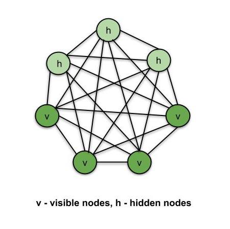
Boltzmann machine is an unsupervised neural network in which each node is connected to every other nodes. It is not a usual neural net. A usual neural net can have fully connected layers, but not intra-layer connection. And the connection in a usual neural net is forward, in a Boltzmann machine, the connection is bidirectional. In a Boltzmann machine, the nodes are classified as visible nodes and hidden nodes. The visible nodes are the ones that can be measured and hidden nodes are the ones that will not be measured. Those two types of nodes are considered in one single system.
Apart from that, a Boltzmann machine is also not deterministic, it is stochastic or generative. It is like a system that learns from data to become a representation of it. With that, it can tell the abnormalities in the system or be a PCA or dimensionality reduction technique.
The network of units would be measured with total energy for the overall network. The units are binary and the weights are stochastic. Here is the energy of the network:
\[E = - ( \sum_{i < j} w_{ij} s_i s_j + \sum_i \theta_i s_i)\]with \(w_{ij}\) is the connection strength between unit j and unit i, \(s_i \in \{0,1\}\) is the state of unit i, \(\theta_i\) is the bias of unit i in the global energy function.
The network runs by repeatedly choosing a unit and resetting its state. Running long enough at a temperature, the probability of a global state of the network depends only on that state’s energy, according to a Boltzmann distribution, not the inital state. We say the machine is at thermal equilibrium, the probability distribution of the global states converges.
Technically, each unit of the Boltzmann machine is a binary unit (it can be in state 0 or state 1). Each unit (state) is in the state space \(\{0,1\}^N\). On that state space, we can define a probability distribution by defining energy for each state and we have the Boltzmann distribution. A Gibb sampling would be a process that sample a sequence from the distribution of these states across the state space that roughly reflects the probability distribution. So we want most of the sequence to be in the regions of the state space with high probability (low energy) and few to be in low probability regions (high energy).
Restricted Boltzmann machine (RBM)
Restricted Boltzmann machine is the Boltzmann machine with the restriction that there is no intra-layer connection. So visible layer would be input layer, and hidden nodes would be hidden layers. In image processing, each input unit is for a pixel of the image. There is no output layer.

Each visible node takes a low level feature from an item in the dataset to learn. The result is fed into an activation function which then produce the node’s output. This is also called the strength of the signal passing through it. The restricted Boltzmann machine is like a standard feed forward fully connected and deterministic neural network.
A RBM can also be considered probabilistic graphical models, or stochastic neural network. In other words, a restricted Boltzmann machine is an undirected bipartite graphical model with connections between visible nodes and hidden nodes. It corresponds to the joint probability distribution:
\[p(v,h) = \frac{1}{Z} exp(-energy(v,h)) = \frac{1}{N}exp(v'Wh + b'v + c'h)\]Then we can perform stochastic gradient descent on data log likelihood, with stopping criterion.
Deep belief network (DBN)
When we stack restricted Boltzmann machines together, we have the deep belief network. The DBN extract features from the input by maximalizing the likelihood of the dataset. A deep belief network is a model of the form:
\[P(x, g^1, g^2.. g^l) = P(x\mid g^1) P(g^1 \mid g^2) ... P(g^{l-1}, g^l)\]with \(x = g^0\) to be input variables and g to be the hidden layers of causal variables.
Each \(P(g^{l-1}, g^l)\) is an RBM:
\[P(g^i \mid g^{i+1}) = \prod_j P(g_j^i \mid g^{i+1})\] \[P(g_j^i \mid g^{i+1}) = sigmoid(b_j^i + \sum_k^{n^{i+1}} W_{kj}^i g_k^{i+1})\]We can train a deep belief network with greedy layer wise training, proposed by Hinton.
Greedy layer-wise training
Learning is difficult for densely connected, directed belief nets with many hidden layers since it is difficult to infer the conditional distribution of the hidden activities given a data vector. But we can train layers sequentially starting from the input layer. Since \(P(g^1 \mid g^0)\) is intractable and we approximate with \(Q(g^1 \mid g^0)\). We treat the two bottom layers as an RBM and fit parameters using contrastive divergence. That would give an approximate \(\hat{P} (g^1)\). We need to match it with \(P(g^1)\). Then we can approximate \(P(g^l \mid g^{l-1}) \approx Q(g^l \mid g^{l-1})\). Each layer learns a higher level representation of the layer below, by treating layers l-1 and l as an RBM. Then we fit parameters using contrastive divergence. Then we sample \(g_0^{l-1}\) recursively using \(Q(g^i \mid g^{i-1})\) starting from \(g^0\).
Contrastive divergence is a training technique that approximate the gradient of the log likelihood based on a short Markov chain (a way to sample from probabilistic odel) starting from the last example seen. It is an approximate Maximum Likelihood learning algorithm.