RL: Deep Q-learning
Introduction
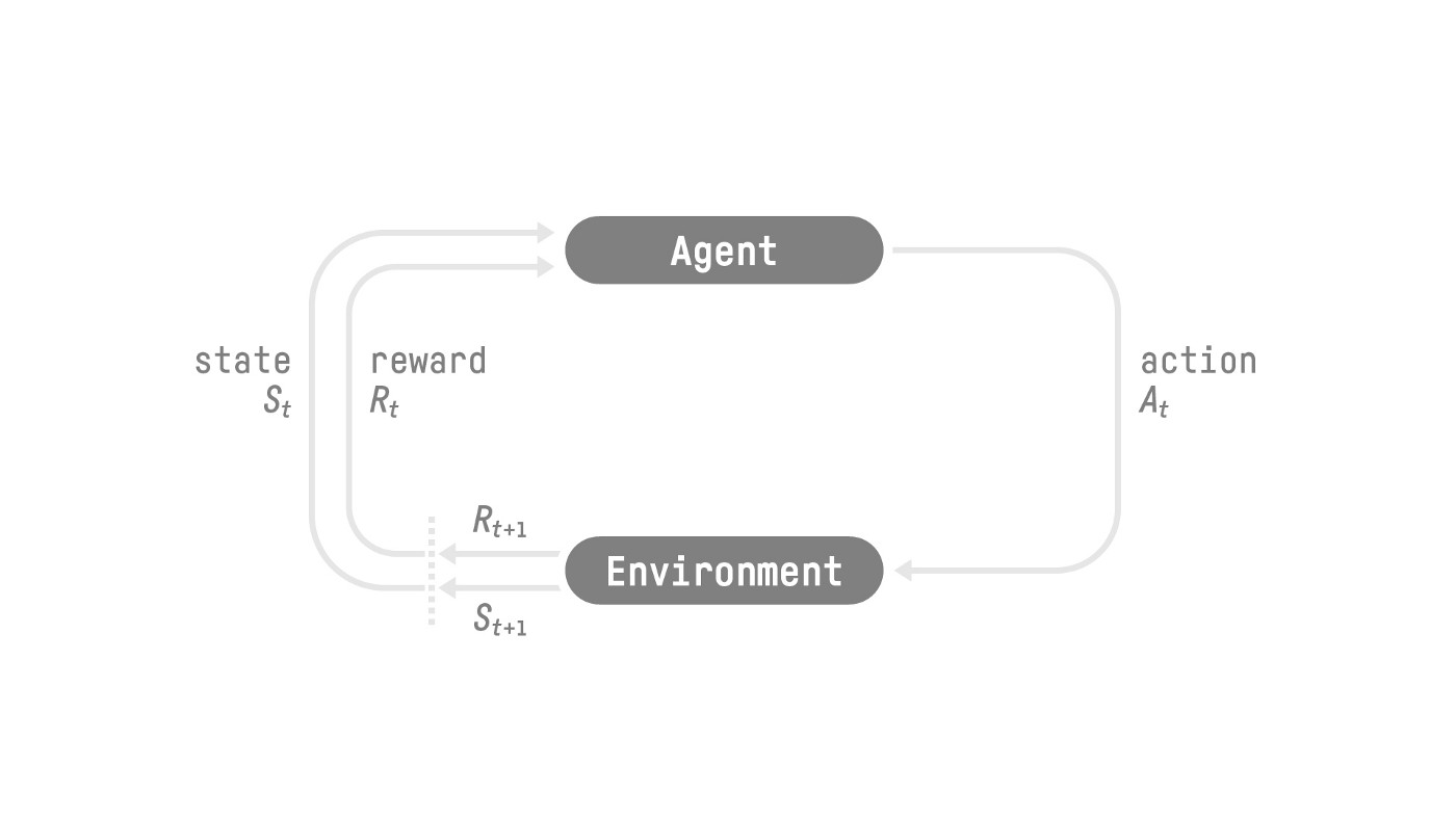
Reinforcement Learning (RL) is the kind of learning that agent learns to make good decision from interacting with the environment. When interacting with the environment, agent receives reward or penalty and adjust their action based on that. This feedback system lets the agent learn from the experience and improve their decision making ability.
There are several key components in reinforcement learning:
- Agent: The learner/decision maker in the environment
- Environment: The simulated world in which the agent operates
- Action A: The possible moves that the agent can make. It can be discrete or continuous.
- State S: The situation that the agent is in
- Reward R: Feedback from the environment that guides the agent towards achieving goal. At each step, the cumulative reward equals the sum of all rewards in the future, with discount \(R = \sum_{k=0}^{\infty} \delta^k r_{t+k+1}\)
- Policy \(\pi\): A strategy/plan to determine action at each state
The goal of the agent is to maximize its cumulative reward (expected return). Sometimes a RL process can be considered a Markov Decision Process (MDP). A MDP cares only about the current state to decide the action, not all the history of all the states and actions.
The policy \(\pi\) is the function that needs to be learned. It is the function that returns an action for any states in the process. The function will be trained to maximize the expected return.
A policy based training algorithm would aim to return action at each state \(a = \pi(s)\). In a stochastic setting, the output is a probability distribution over actions \(\pi(a\mid s) = P(A\mid s)\). Using deep learning, we can approximate the policy with a neural network.
A value based training algorithm learns a value function that maps each state to the expected value of that state. The expected and discount value of that state is the cash flow that the agent would get if follows the path from that state and each time choose the state with highest value (a greedy policy).
\[v_{\pi}(s) = E_{\pi}{[R_{t+1} + \delta R_{t+2} + \delta^2 R_{t+3} + ... \mid S_t = s ]}\]Using deep learning, we can approximate the value function with a neural network.
Find an optimal value function would lead to an optimal policy.
\[\pi^*(s) = arg max_a V^*(s,a)\]One thing to know about RL is that there needs to be a consideration between exploration and exploitation. Exploration is to explore the environment by trying random actions. This is to learn more about the environment in general. Exploitation is when we don’t care about getting to know the environment, but use the what information we have to maximize the reward. Sometimes if we only do the exploitation (care about the immediate rewards), we miss the path leading to a big amount of reward down the line. So, as an extension, we can use an epsilon-greedy policy that choose the highest value but sometimes (\(\epsilon\) probability) explore random option.
For the value-based method, there are two types of functions: state value function and action value function. The state-value function calculates the expected return if the agent is in that state:
\[V_{\pi}(s) = E_{\pi} {[G_t \mid S_t = s ]}\]The action value function calculates for a pair of state and action the expected return if the agent is in that state and take the action (so the expected value for taking that action in the state).
\[Q_{\pi} (s,a) = E_{\pi} {[G_t \mid S_t = s, A_t = a ]}\]The Bellman equation lets us calculate the value for each state to be the immediate reward of that state and the discounted value of the next one:
\[V_{\pi}(s) = E_{\pi} {[R_{t+1} + \delta V_{\pi}(S_{t+1}) \mid S_t = s ]}\]Let’s explore two strategies on training value function: Monte Carlo and Temporal Difference.
Monte Carlo
Monte Carlo method waits for the return of a game play, then use the return as an approximation of the value of the future game.
\[V(S_t) \leftarrow V(S_t) + \alpha{[G_t - V(S_t)]}\]with \(V(S_t)\) being the estimation of value at state t. \(\alpha\) being the learning rate. \(G_t\) being the return at state t. Specifically, we start at the starting point, the agent takes action according to epsilon greedy policy, the agent gets the reward and the next state. The termination rules is when the agent reaches the goal or if it has been more than N steps. At the end of the game, we have a list of state, action, reward, and next state. We sum up the total reward \(G_t\), then we update \(V(s_t)\) based on the above formula. After repeatedly play the game, the agent will learn.
Temporal Difference learning
Temporal difference (TD) method waits for one interaction \(S_{t+1}\) and update the value of the state using the immediate reward and the discounted value of the next state. TD updates \(V(S_t)\) at each step. We don’t have \(G_t\) but we estimate \(G_t\) with the immediate return and the discounted value of the return of the next state. This method is called bootstrapping.
\[V(S_t) \leftarrow V(S_t) + \alpha {[ R_{t+1} + \delta V(S_{t+1}) - V(S_t) ]}\]Q-learning
Q means quality (value). Q-learning is an off-policy value-based method that uses TD to train for its Q-function (an action-value function). Off-policy means using a different policy for acting and training (update the Q-value to rethink the policy). When we actually choose the action, we use the epsilon greedy policy (sometimes explore), but when we calculate to update the policy we use the greedy policy (only exploit - choosing the maximal possible value).
The training of the Q-function would end up to be a Q-table that contains all the state-action value pairs. After training, we would have an optimal Q-function, Q-table, so that each time, for a state and action pair, Q-function can search the Q-table for the value. With optimal Q-function, we have optimal policy.
The algorithm goes as follows, first we initialize the Q-table (values for each state-action pair). At each step, we choose action according to epsilon-greedy policy: we do exploitation (selecting the highest value action) at probability \(1 - \epsilon\) and do exploration (trying random action) at probability \(\epsilon\). \(\epsilon\) changes with time, at the begining we can choose to explore a lot, but when the Q-table gets better, we gradually reduces \(\epsilon\). Second, after choosing action \(a_t\), the agent gets the feedback from the environment, to receive reward \(r_{t+1}\) and the information on the next state \(s_{t+1}\).
Similar to the value equation, we update \(Q(s_t, a_t) \leftarrow Q(s_t, a_t) + \alpha {[R_{t+1} + \delta max_a Q(s_{t+1}, a) - Q(s_t, a_t) ]}\). Note that after getting the reward \(r_{t+1}\), we use a greedy policy (choose the next best action). After updating the Q-value, we start in a new state and use a epsilon greedy policy again.
Deep Q-learning
When the number of the states grow big, using Q-table becomes ineffective. We can use a neural network instead of a Q-table to approximate Q-value for each action in each state. For example, to train a RL to play Atari game, first we stack 4 frames of the game together. This is to capture information on time (movement and direction). We can use a neural network of three convolutional layers, to analyze spatial relationships in those images. Then there are some fully connected layers that flatten the convo matrix and output a Q-value for each action at the state.
There would be a loss function that compares the Q-value prediction and the Q-target, so that gradient descent can be used to update the weights of the deep Q-network to predict Q-values better.
\[Q-target = R_{t+1} + \delta max_a Q(S_{t+1}, a)\] \[Q-loss = R_{t+1} + \delta max_a Q(S_{t+1}, a) - Q(S_t, A_t)\]To use the experiences of the training better, a replay buffer is used to save experience samples so that those can be reused. In this case, same experience can be relearned. We can also fix a Q-target network to be trained separately.
We can use a neural network called Q-network consisting of a series of dense layers for the Cart Pole problem, with Adam optimizer.
fc_layer_params = (100, 50)
action_tensor_spec = tensor_spec.from_spec(env.action_spec())
num_actions = action_tensor_spec.maximum - action_tensor_spec.minimum + 1

# Define a helper function to create Dense layers configured with the right
# activation and kernel initializer.
def dense_layer(num_units):
  return tf.keras.layers.Dense(
      num_units,
      activation=tf.keras.activations.relu,
      kernel_initializer=tf.keras.initializers.VarianceScaling(
          scale=2.0, mode='fan_in', distribution='truncated_normal'))

# QNetwork consists of a sequence of Dense layers followed by a dense layer
# with `num_actions` units to generate one q_value per available action as
# its output.
dense_layers = [dense_layer(num_units) for num_units in fc_layer_params]
q_values_layer = tf.keras.layers.Dense(
    num_actions,
    activation=None,
    kernel_initializer=tf.keras.initializers.RandomUniform(
        minval=-0.03, maxval=0.03),
    bias_initializer=tf.keras.initializers.Constant(-0.2))
q_net = sequential.Sequential(dense_layers + [q_values_layer])

optimizer = tf.keras.optimizers.Adam(learning_rate=learning_rate)

train_step_counter = tf.Variable(0)

agent = dqn_agent.DqnAgent(
    train_env.time_step_spec(),
    train_env.action_spec(),
    q_network=q_net,
    optimizer=optimizer,
    td_errors_loss_fn=common.element_wise_squared_loss,
    train_step_counter=train_step_counter)

agent.initialize()
You can check out the result here
Conclusion
In conclusion, Deep Q-Learning, a powerful combination of Deep Learning and Reinforcement Learning, has revolutionized the field of artificial intelligence, enabling machines to learn complex behaviors without explicit supervision. By directly learning the optimal policy from high-dimensional inputs, Deep Q-Learning has opened up new possibilities for AI applications, from game playing and robotics to autonomous driving and beyond.