Stacking
TOC
Stacked generalization
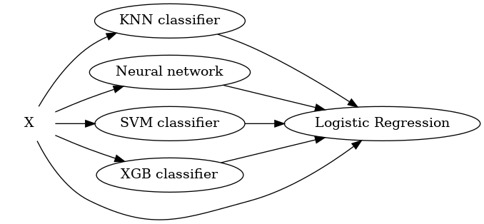
Stacking, also called stacked generalization, is one of the popular techniques of ensembling. Similar to bagging and boosting, stacking also combines prediction from multiple base models, trained on the same training set. This is to take advantage of the fact that different models have very different internal representations, say, Linear Regression and Random Forest. Hence they have different skills and if we can combine those expertise we can achive something better. The difference of stacking with bagging is that stacking uses many different machine learning model, instead of only decision tree. And then all the base models are trained on the training set, instead of sampling from those training set. The difference with boosting is that stacking uses a new model to combine the prediction, instead of predict the error of the previous model. In general, stacking is like a more sophisticated version of cross validation.
A general stacking model includes two levels: base models and the meta model:
-
Base model learns directly from the training set. The outputs would be used as input for the meta model. The base models can be any models: decision tree, SVM, neural network.. Since the way they learn are different, the outputs and errors are not correlated. To avoid overfitting, we can use k-fold cross validation technique.
-
Meta models use the output of base models as their input and output a prediction, with respect to the labels of the problem. This is how the predictions of base models are combined. The meta models can be simple techniques: linear regression to output a real value for the regression task, and logistic regression to output a label probability for the classification task.

The drawback is that the computation time increases with the number of base models.
Variants
K fold cross validation
The algorithm for basic stacking:
- Level-0: learn directly from the original dataset:
- For \(t \leftarrow 1\) to T do:
- Learn a base classifier \(h_t\) based on dataset D
- For \(t \leftarrow 1\) to T do:
- Construct new dataset from D:
- For \(t \leftarrow 1\) to m do:
- Construct a new dataset that contain \(\{x_i^{new}, y_i\}, x_i^{new} = \{h_j(x_i) \mid j = 1 \to T \}\)
- For \(t \leftarrow 1\) to m do:
- Level-1: learn a new classifier based on the newly constructed dataset
- Return \(H(x) = h^{new}(h_1(x), h_2(x)...h_T(x))\)
Given a dataset with N observations \(D = (x_n, y_n), n = 1,..N\) where \(y_n\) is the class value and \(x_n\) is the attribute vector of the n instance. Let’s split the data into K parts: \(D_1,...D_J\). As an usual K fold cross validation task, let \(D_j\) will be the test set and \(D^{(-j)} = D - D_j\) to be the training set for the kth fold. Now we assemble L learning algorithms, which are called level-0 generalizers. Each learning algorithm l will train on the training set \(D^{(-j)}\) and result in the model \(M_l^{(-j)}\). At the end, the final level-0 model \(M_l, l = 1,...L\) is trained on all the data in D.
For the test set, for each \(x_n \in D_j\), let \(z_{ln}\) be the prediction of \(M_l^{(-j)}\) on \(x_n\). After doing all the cross validation, the dataset assembled from the outputs of the L models would be \(D_{CV} = \{(y_n, z_{1n}, ...z_{Ln}), n = 1,...N \}\). This is called the level-1 data since it is the output of all the level-0 models.
We then decide on a level-1 generalizer to derive from that level-1 dataset: the model M for y as a function of \((z_1, ...z_L)\). This is called level-1 model.
For the classification process, \(M_l\) will be used together with M. For a new instance, model \(M_k\) will output a vector \((z_1,...z_K)\). This vector is then be the input for the level-1 model M, who will output the final classification result for that instance. This is the original stacked generalization process.
Apart from the hard classification, the model also considers probabilities of classes. Assume I classes. For model \(M_l^{(-j)}\) and instance x in \(D_j\), the output of the model is the probability vector for nth instance: \(P_{kn} = (P_{k1}(x_n),...P_{kI}(x_n))\) for \(P_{ki}\) to be the probability of the ith output class.
The level-1 data would be all the class probability vectors from all L models, together with the true class:
\[D'_{CV} = \{(y_n, P_{1n}, ... P_{Kn}), n=1,...N \}\]The level-1 model trained on this dataset would be called M’.
There are reasons why stacking in this way works to improve the overall performance. First, each base model will add to the coverage of the training set. For example, base model 1 can cover 60% of the dataset, base model 2 can cover 30%. Together they can cover at most 90%, and in their special ways. Second, using a meta learner can describe the output of all base models in non trivial way, instead of just choosing winner-takes-all or simple average method. In the case of winner takes all, if we simply choose the highest confident output, it is just like using that base learner alone, we haven’t utilized the other base learners and their sophistication. Similarly, taking average of the outputs of the base learners also fail to take into account the intricacies of each learners. By doing the combination in a sophisticated way, we combine the output better and increases overall performance.
Restacking
One way to improve the stack is to pass the original training set altogether with the outputs of the base models into the next level learner. In this method, the output predictions by the base models are considered new data points, and they can be concanated with the original data points to form a new dataset for the training of the meta model.
Aggregate test predictions
We can generate multiple test predictions and average them ( or use hard voting in the case of classification task) for the prediction of the test set. The difference with usual stacking is that, in each run, at the end of the cross validation step, the base model will not be trained for the entire original set before getting prediction on test set, but it would be trained for the fold only, therefore there will be L test predictions. We then aggregate those for a final unique test prediction for each base model. So, with k-fold and m base models, the number of predictions on the test set during training will be \(k*m\) times (again, each base model will predict k times on the test set). This helps in improving accuracy and reduce overfitting but it increases the computational cost. The cost would become significant for large dataset.
Multi-level stacking

Apart from the only level-1 meta learner, we can add more level-1 meta learners and then we add level-2 learners as well, before coming to the final prediction.
Variants of meta learner
Voting scheme
This is probably the simplest stacking ensemble method, in which all the member models are prepared individually and the final result uses simple statistics (mean or median) instead of learning. When we choose the prediction with highest number of votes, it is hard voting. And when we sum the probabilities of all voters, it is called soft voting. By doing the voting, all base models are considered to be equal (i.e. having the same skill level).
Weighted average
A basic approach in this direction is to weigh each member model based on its performance and try those on a hold-out dataset. It can also help to tune the coefficient weightings for each model using an optimization algorithm. The final prediction would be a combination of all member’s prediction, but weighted accordingly with each member’s confidence and performance.
Blending ensemble
When k-fold cross validation seems to be a complicated option, we can do blending. In blending, we divide the training set into subset 1 and subset 2. N base models would train on the subset 1, then they predict on subset 2. The subset 2 together with base models’ predictions would be used as input to train the meta model.
Super leaner ensemble
The reason this is called super learner is that it incorporates all the above techniques.
-
First it splits data into V blocks. Then for each block, it train many base models. The learned base models then are used to predict the outcomes in the validation set. Then we perform model selection and regression fitting on all the outcomes of the base models.
-
Second it train each base model on the entire dataset (like in the original stacking algorithm).
-
Finally the super learner is the combination of predictions from each base leaner in the first and second step.
Code example
We would try KNN, SVM, and Random Forest as base models. We use the StackingRegressor from sklearn to be the stacking method, the final estimator is a linear regression with 5-fold cross validation.
We achieve better MSE (mean squared error) with the stacked ensemble: 52 in comparison with 54, 55 and 67. But the stacked model runs in much longer time: 8 seconds in comparison to less than 2 seconds.
from sklearn.datasets import load_diabetes
from sklearn.model_selection import train_test_split
from sklearn.linear_model import LinearRegression
from sklearn.neighbors import KNeighborsRegressor
from sklearn.svm import SVR
from sklearn.ensemble import RandomForestRegressor, StackingRegressor
from sklearn.metrics import mean_squared_error
import timeit
import time
X, y = load_diabetes(return_X_y=True)
X_train, X_test, y_train, y_test = train_test_split(X, y, random_state=42)
base_models = [
    ('KNN', KNeighborsRegressor()),
    ('SVR',SVR()),
    ('Random Forest',RandomForestRegressor()),
    ]
stacked = StackingRegressor(
    estimators = base_models,
    final_estimator = LinearRegression(),
    cv = 5)
for name, model in base_models:
    start_time = time.time()
    model.fit(X_train, y_train)
    prediction = model.predict(X_test)
    end_time = time.time()

    r2 = model.score(X_test, y_test)
    rmse = mean_squared_error(y_test, prediction, squared = False)

    print("-------{}-------".format(name))
    print("Coefficient of determination: {}".format(r2))
    print("Root Mean Squared Error: {}".format(rmse))
    print("Computation Time: {}".format(end_time - start_time))
    print("----------------------------------\n")
start_time = time.time()
stacked.fit(X_train, y_train)
stacked_prediction = stacked.predict(X_test)
end_time = time.time()
stacked_r2 = stacked.score(X_test, y_test)
stacked_rmse = mean_squared_error(y_test, stacked_prediction, squared = False)
print("-------Stacked Ensemble-------")
print("Coefficient of determination: {}".format(stacked_r2))
print("Root Mean Squared Error: {}".format(stacked_rmse))
print("Computation Time: {}".format(end_time - start_time))
print("----------------------------------")
-------KNN-------
Coefficient of determination: 0.44659346214225026
Root Mean Squared Error: 55.31877155619498
Computation Time: 0.030904293060302734
----------------------------------

-------SVR-------
Coefficient of determination: 0.18406447674692117
Root Mean Squared Error: 67.17045733565952
Computation Time: 0.02379894256591797
----------------------------------

-------Random Forest-------
Coefficient of determination: 0.46919179281278434
Root Mean Squared Error: 54.17752973261081
Computation Time: 0.14402318000793457
----------------------------------

-------Stacked Ensemble-------
Coefficient of determination: 0.5108685440878455
Root Mean Squared Error: 52.00716509859344
Computation Time: 0.7904818058013916
----------------------------------